I have 10 students. Deselect Select All. We want to return lucky lottery numbers. This will generate a random number between 0 and 1. Lets fix this. In an unused column to the right, use this formula in row 2, =C2+B2/1000 Fill down as necessary. MATCH () Excels MATCH () function will return the relative location of the first occurrence that satisfies the match criterion (the lookup_value) within the specified array (the lookup_array). 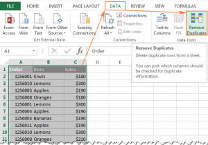 The result is 1, because Sweater is item number 1, in that range of cells.
The COUNTIFS function lets us count based on multiple criteria, so well use that to create an Excel Rank IF formula. Start and Step default to 1, if omitted. The ref is the cell range that contains the list of numbers you want to compare it to. The first column now contains a list of unique numbers in random order. errors);; list is the range of numbers that are to be ranked.This should be a column or row vector (i.e. Insert the formula: =COUNTIFS (Store,C3,Sales,">"&D3)+1. Note: the +1 at the end of the formula is required to start the ranking at  RANK.AVG gives same rank to duplicates like a rank function but it averages and may give decimal ranks to duplicates. Press Enter to get the count. If there is an duplicate score, the 2 score will share the same rank, e.g rank 5, the next rank will be rank 6, but per your formula, it will skip rank 6 and go to rank 7. 6 instead of rank 7. The problem I have with it is that it returns duplicates, because for 2 or 3 cells, the first best match is the same, until my search area has moved down enough to continue on to the next match. Multiple change-point models are here viewed as latent structure models and the focus is on inference concerning the latent segmentation space We can blend measures by dragging the 1st measure on one axis and 2nd on the existing axis Select the Data tab, then click the Filter command To change the width of all columns, first select Cell G4 has the following function: Conclusion. Get the rank with criteria using COUNTIFS function. Count duplicates. The formula that goes in G2 is:
Lets get started and dive right in. The rank for Jan 2nd is 1. To remove excel duplicates, click on the filter drop-down icon in the column header. A further advantage of these formulas over RANK is that they work on text strings, where they sort alphabetically, as well as numbers. In the example shown below, highlighted ones are the students with their same scores.
To rank items in a list using one or more criteria, you can use the COUNTIFS function.
We move over to RANK.AVG function. As you can see from the results in the image above by using the RANK function, it turns out that we find that there are multiple rankings in the ranking results.
Rename the Index column to Rank. Example generate non-duplicated random number. Pull down the fill handle (located at the bottom right corner of the cell) to copy the formula to as many cells as you need. So here is the scenario. Click on Conditional Formatting Highlight Cells Rules Duplicate Values . In the example shown, the formula in E5 is: = COUNTIFS( groups, C5, scores,">" & D5) + 1. where "groups" is the named range C5:C14, and "scores" is the named range D5:D14. So, I found your site as I couldn't get AND to work to use multiple IF criteria in an INDEX/SMALL formula. This worked perfectly!
The syntax is the same as RANK. As the result, for all 1st occurrences, COUNTIF returns 1, from which you subtract 1 to keep the original ranking. For 2nd occurrences, COUNTIF returns 2. By subtracting 1 you increment the ranking by 1, thus preventing duplicate ranks. For example, for B2, RANK.EQ returns 1. As this is the first occurrence, COUNTIF also returns 1. Step 4: Now we will select the Range of selected cells or columns A. Lookup the Second, Third, or Nth Value in Excel. Figure 5: The duplicate wording in our ranking list has been removed.
You can generate multiple rows and columns. In the given situation, you can see that we have a lot of rows containing text, though duplicates are coming in these lines. For descending rank : In cell D3, type the following formula. So here is the scenario. Since the whole point of this exercise was to Identify Duplicates but not remove the duplicate records, were still not in a good place. On the Ablebits Tools tab, click Randomize > Select Randomly. Figure 2: Unique Values Option. Step 1: Go to cell D1 and enter this formula = SUMPRODUCT (1/COUNTIF ( B1:B11,B1:B11)). Select the cell B2, drag the fill handle down to the cell B11, then the unique ranking is finished. Step 3: Identify Duplicates and Show Duplicate Records. Example of desired outcome: Multi-criteria sorts can be achieved by adding COUNTIFS. Heres the data you have: The criteria are Name and Product, and you want them to return a Qty value in cell C18. The RANK function does exactly this and it supports ranking unsorted data, assigning ranks in either ascending order or descending order. If you add "--" before the bracket, it will return "1" or "0" respectively for "True" or "False", thus making it easier for calculating (counting, for example). (This is where the ranking occurs). Code: Sub VBARemoveDuplicate1 () Selection.End (xlDown).Select End Sub. In this article, we will learn how to lookup for multiple value with duplicate lookup values in Excel. COUNTIFS expands on what the COUNTIF function does and allows you to use multiple criteria. If sorting by row, click "Options" and select "Sort left to right." I prepared an exam. In the Allow list, click Custom. Step 3: In the process of removing the duplicate, first we need to select the data. The RANK function does a good job of indicating the scores in order of first, second, third, and so on. Formula 2: Match the Duplicate Values with INDEX, ROW, and SMALL. Figure 1: Duplicate Values. As you can see all the different duplicates are marked which proves the formula works fine. In that exam each student scored marks out of 100. Define the sample size: that can be a percentage or number. 4 Responses to "Excel : Lookup Top N values ignoring duplicates" Hi Thanks for the file. Press Enter. To get that, we first need to find all of the rows that match the car that were looking for, then we will simply move 1 cell to the right to get the name of the owner. So if you want 10 random numbers, copy it down to cell A11. For example, as shown above, in a list of integers sorted in ascending order, the number 100 appears twice with a rank of 4. Step 2: We need to specify logical criteria under AND function.
This example teaches you how to use data validation to prevent users from entering duplicate values. The condition (or conditions) that you want to apply. To fix this, we subtract by the number of duplicates + 1 (2-1 = 1). The formula in Cell E10 is: {=SUM (-- (COUNTIF (B2:B8,A2:A7)>=2))} As the logic statement requires values greater than or equal to 2, it will only count the duplicates. Behind the scenes it gives each duplicate a rank, and then finds the average for them. Cell J4 contains the name of the city; London or Birmingham. On the Data tab, in the Data Tools group, click Data Validation. Step 1: In cell E1, as we need to check how AND operator works for multiple criteria, start initiating the formula by typing =AND (. However, in the case of ties this will give you 1, 3, 3, 4 instead of 1, 2, 2, 4. Re: Ranking with multiple criteria and eliminating duplicates Hello, For lots of IF statement, (this = that, there > here, etc), it will often return boolean values (True / False).
Excel built-in data sorting is amazing, but it isnt dynamic. This first would be this formula, which will rank everything with a unique rank (first appearance of 14 gets ranked 4 and the second appearance gets ranked 5): The simplest use of ranking is to get the rank of one or more values in a list. First, sort the data in ascending order on which you want to calculate the ranking. 5 and the next score will flow to rank no.
Click new rule.. However, since Excel 2010, two additional rank functions have been added, namely, RANK.AVG and RANK.EQ. Oftentimes it is necessary to use multiple columns to obtain a ranking, either because the business requirement dictates it, or because you want to rank ties with different criteria. Using array formulas. Right now my formula gives the same ranking for the same value (views it as a tie and ranks it as such). In earlier versions of Excel, only the RANK function was available. For ascending rank : In cell E3, type the following formula. Note the the RANK function by itself will assign the same rank to duplicate values, and skip the next rank value. When the Data is all Text with No Duplicates. It also takes into consideration the impact of negative and positive numbers and ranks them appropriately. Go to the Data tab in the Excel Ribbon. Notice that rows 5, 8, and 21 have a rank of #2 while rows 6 and 10 have a rank of #3; rows 7 and 17 have a rank of #4. The work around is to use an Excel Array Formula. Step 2: In the Home tab, select conditional formatting from the styles section. Now in Excel, i want to write a formula that tells me top 5 scorers name. It still compares the number to its position in the list and it skips values. However, the presence of duplicate numbers affects the ranks of subsequent numbers. Read more articles by David Ringstrom. In this article, we will learn how to lookup for multiple value with duplicate lookup values in Excel. The condition (or conditions) that you want to apply. There is no RANKIF function in Excel. From the displayed results (6) we can see there are no duplicates. Can guide the formula if we want same score with same rank as rank no. Sort the Item column in ascending order (to rank ties alphabetically) Go to Add Column --> Index Column --> From 1. Search: Excel Filter Multiple Columns Simultaneously. Step One: Create a Helper Column to Calculate Relative Rank. Hi reviving this as I've got a bit of an issue using INDEX and IFs. Lets take an example to understand. Then, rank each player based on assists. Step 3: Sort the column of random numbers. Click on the down arrow and select Unique as shown in figure 2 below. You can see this in the Rank 1 column, rows 8 and 9 in the worksheet. Apply the formula =RANK.EQ ($B2,$B$2:$B$8)+COUNTIFS ($B$2:$B$8,$B2,$C$2:$C$8,">"&$C2) to cell D2. Drag the formula down to the other cells in the column by clicking and dragging the little + icon at the bottom-right of the cell. (This is where the ranking occurs). Select cell D5 and enter the following formula: =SUMPRODUCT ( (B5<=$B$5:$B$24)/COUNTIF ($B$5:$B$24,$B$5:$B$24)) Fill the formula down the remainder of the table. About the author: Press enter. In that exam each student scored marks out of 100. Select cell B2, copy and paste formula =RANK (A2,$A$2:$A$11,1)+COUNTIF ($A$2:A2,A2)-1 into the Formula Bar, then press the Enter key. I have been trying to work out a Ranking method wherein the Duplicate values are retained without skipping sequence. (4+5+6)/3 = 5, hence will give the rank of 5 for all 3. 1. Deselect Select All. where: number is the value to be ranked.It should be noted that the RANK value only works with numbers (this is why the last rank in the example below is #N/A the value is a blank cell; text will create #VALUE! The answer is hidden in the question itself, as you only have to use UNIQUE Function in it & type instead of =COUNTA (D5:D20), =COUNTA (UNIQUE (D5:D20)), then we will get the result as 4, which is what we require. I prepared an exam.
If sorting by column, select the column you want to order your sheet by. In the first cell (A2), type: =RAND (). Rank duplicate without skipping numbers.
Rank 4 have 2 duplicate. RANK.EQ gives duplicate numbers the same rank. Thank you! =SEQUENCE (rows, columns, [start], [step]) In the first example below, this formula returns a sequence of numbers in 1 row and 5 columns. Now copy the formula in other cells using the drag down option or using the shortcut key Ctrl + D as shown below. Since this column is random, the sort order applied to the first column will be completely random. =SEQUENCE (2,3,10,5) Go to the Data tab in the Excel Ribbon. Hence, if you have 4th rank for 3 values, it will average 4, 5 and 6 i.e. Select the row right below the row or rows you want to freeze In the next tutorial, Extend Data Model relationships using Excel 2013, Power Pivot, and DAX, you build on what you learned here, and step through extending the Data Model using a powerful and visual Excel add-in called Power Pivot Move into to worksheet, Nested LARGE with ROW function to automatically increments the rank position. The top 10 will only be returned for customers in that city. The rank of a number in a list is the position at which the value would be placed if the data list were sorted. Rank returns a computed rank, which will include ties when the values being ranked include duplicates. This will add a new field in your pivot with a value of 1 in all cells. We will first generate a 1-10 numerical ranking of the information we want sorted. To rank multiple values based on criteria, we use the COUNTIFS function and the SUMPRODUCT function of Excel. RANKIF is basically a conditional rank. The result is a rank for each person in their own group. Andrew - this appears to work: =RANK($G2,$G$2:$G$22,1)+SUMPRODUCT(($G$2:$G$22=$G2)*($F$2:$F$22<$F2)) As you can see from the first value returns, the first duplicate means this value as other duplicates. In any case, as shown in Figure 5, bananas no longer appear on the list twice. range is the array that you wanted evaluated by the criterion (in this instance, cells F12:F21); criterion is the criterion in the form of a number, expression, or text that defines which cell(s) will be added, e.g. A dropdown arrow will appear beside the column header. Because the value that you want to return is a number, you can use a simple SUMPRODUCT () formula to look for the Name James Atkinson and the Product Milk Pack to return the Qty. Step 1: Select the range A2:C8 in the given data table. In this tutorial, I will cover two ways to look-up the second or the Nth value in Excel: Using a helper column. When we grouped our records, we lost both the Brand names column, but also any duplicate records. Alternative solution to break Excel RANK ties Another way to rank numbers in Excel uniquely is by adding up two COUNTIF functions: Use criteria as cell value greater than 16 for all cells (B1, C1, D1). You will see a window shown in Figure 1 below.
Most often, this is what you want. We can use the following formula to perform this multiple criteria ranking: =RANK.EQ ($B2, $B$2:$B$9) + COUNTIFS ($B$2:$B$9, $B2, $C$2:$C$9, ">" &$C2) We can type this formula into cell D2 of our spreadsheet, then copy and paste the formula down to every other cell in This will show duplicated values which you may delete. Using * works fine when I reference some data in the IFs but then completely ignores it if I change the reference. Click on the Filter feature. Preferably without adding more columns, but if there's no other way I'd accept any solution! This only removes unique duplicates, if you start including your date or sales values in the list you find Excel sees only unique values. This ranking method is super easy to create: Sort the Sales column in descending order. After that, open the calculated field dialog box and enter =1 in the formula input bar. 1. This will not rearrange the information, but tell us its place in the list. To calculate rank if, we will use two criteria: Count only the values that are greater than the current rows value. Share The function SUMIF(range,criterion,sum_range) is ideal for summing data based on one criterion:. In this tutorial, I will show you various ways (with examples) on how to look up the second or the Nth value in Excel. One limitation of RANKX is that it is only capable of ranking using a single expression. Two ways you can go about this.
The criteria can include dates, numbers, and text. Approach 3 RANK.AVG Function. This will show Blazone Warriors ahead of Bento All Stars in the rankings.
Click the Data tab, and choose Data Validation from the Data Validation dropdown (in the Data Tools group). So, in our formula: the MATCH function looks for Sweater in the range B2:B4. Step 3: The pop-up window titled new formatting rule appears. You can now use a conventional RANK function on this helper column like =RANK (D2, D$2:D$9) for your ranking ordinals. For this, in VBA we will Selection function till it goes down to select complete data list as shown below. In the resulting dialog, choose Custom from Then the first ranking number is displayed in cell B2. Reorder the columns if desired. Hello there, please i need some support with a rank formula to consider the duplicated values i used this function to rank my value A dropdown arrow will appear beside the column header. A Note about the word Rows. The RANK.AVG Function is new in Excel 2010 and it was intended to create an alternative to duplicate ranks. 3. Re: Multiple Criteria Ranking To Ignore Duplicates. Reply
As seen above, the RANK function gives duplicate numbers the same rank. Note: the +1 at the end of the formula is required to start the ranking at I have 10 students. =SUMPRODUCT ( ($C$3:$C$10>$C3)/COUNTIF ($C$3:$C$10,$C$3:$C$10))+1. However, I'm having an issue with the multiple criteria. Finding the 2nd, 3rd, 4th . i dont want to ignore duplicate, lets say if we have following data: 10, 10, 10, 9, Choose how you'd like to order your sheet. The COUNTIFS form can also be used as an array formula though it requires the criteria ranges to be references and not arrays . =SEQUENCE (1,5) In the second example, the result is a sequence of numbers in 2 rows and 3 columns, starting at 10, with a step of 5. Now in Excel, i want to write a formula that tells me top 5 scorers name. Second, define the upper range of lower range of the random number. 3 Formulas with INDEX-MATCH to Deal with Duplicate Values in Excel. The second part of the formula breaks the tie with COUNTIF: Select the range A2:A20. The first formula with the criteria ($B2,$B$2:$B$8) counts the number of times the values appear. To remove excel duplicates, click on the filter drop-down icon in the column header. DAX offers the RANKX function to compute ranking over a table, based on measures or columns. Navigate to "Data" along the top and select "Sort." Select True and then click on Ok. For example, in a list of integers sorted in ascending order, if the number 10 appears twice and has a rank of 5, then 11 would have a rank of 7 (no number would have a rank of 6). We use Rand function to select a set of 5 random numbers between 1 and 10, without getting duplicates. To solve the double ranking problem and create a unique ranking or ranking for students, it is relatively easy, one way is to use Excels COUNTIF function.
Before running the above VBA, the first thing is to define the Excel Range in which you want to generate random number. Search: Excel Filter Multiple Columns Simultaneously. Add Pivot Table Rank in Excel 2007 and Below. See screenshot:
First, rank each player based on points. These functions will provide you with the same outputs that you are expecting from this article. If a cell is 0 the formula will return a blank cell. To calculate rank if, we will use two criteria: Count only the values that are greater than the current rows value. If there happen to be 3 occurrences of the same value, COUNTIF ()-1 would add 2 to their ranking, and so on. The first COUNTIF function is used to find out the number of values greater or less than the number that is going to be ranked. The second COUNTIF has an expanding range $B$2:B2 and extracts the number of values that are equal to the number. Rank in Excel Using Multiple Criteria Please notice that a duplicate number is also given a rank, though cell B5 is not included in the formula: If you need to rank multiple non-contiguous cells, the above formula may become too long. In this case, a more elegant solution would be defining a named range, and referencing that name in the formula: By subtracting 1 you increment the rank by 1 point, thus preventing duplicates.
Note: The new rule option helps highlight a specific count of duplicates using the COUNTIF formula. The result is 10, from row 1 in that range. Formula 3: Extract Data Based on Duplicates in Two Columns with INDEX+MATCH. But there is still an issue here. Adding criteria. Select True and then click on Ok. All matching rows of cars will have the corresponding owners in the next cell and this is how we will get our unique list. For example, you can ask Excel to count the number of times Paul Jones appears in a range, or the number of A Jones that appear. 2. The syntax for RANK is as follows: = RANK ( number, ref, [order]) In Excel 2010 and newer, RANK has been re-named to RANK.EQ with the same syntax: = RANK.EQ ( number, ref, [order]) The number is the value you want to find the rank for. View best response. Toms Tutorials For Excel: Ranking With Ties. Download Practice Workbook. COUNTIF The COUNTIF function in Excel counts the number of cells within a range based on pre-defined criteria. On the add-in's pane, do the following: Choose whether you want to select random rows, columns, or cells. The outside IF(LEN(D3), , "") wrapping function avoids errors. the INDEX function looks in the range C2:C4. By applying the same formulas, but changing the logic threshold we can calculate the number of duplicate values. If there is a change in the number or positions of # columns, then this can result in wrong data With it, you just need to select the criteria as same as using the Filter feature without typing the criteria manually To freeze header row, freeze multiple rows, unfreeze panes, freeze multiple columns, etc He can select all or any of The COUNTIF function is an incredibly versatile function, in this case, instead of counting values based on a condition we simply check if a value is smaller or larger than the others. Step 1 - Calculate rank. You may have come across situations where you need to rank a series of numbers, such as a list of test scores or elapsed times in a footrace.
Here's what I'm using: =COUNTIFS(D:D,D2,H:H,">"&H2)+1 Column D - groups Column H - value that is being ranked Looking to consecutively rank column H, based on column D's group, without duplicates/ties! Nested LARGE with ROW function to automatically increments the rank position. The last step is to apply filters to both columns and sort the column that contains the random numbers. Let's explore their differences, as you'll likely see them all in Excel. This use of COUNTIF gives you an effective means to break ties when necessary within your Excel spreadsheets. The ranking order is from highest to lowest number.
To return the random numbers, avoiding duplicates, we will use Rand, Rank and VLOOKUP function along with row function. Highlight the rows and/or columns you want sorted. Figure 5. In our example file, look at the Top 10 non-DA with criteria tab. Drag the formula to the cells below. Remember, we are using text values so the function returns a rank number based on the position if the list were sorted alphabetically. The default option selected is Duplicate . This means you can add data, and it will automatically sort it for you. If you want to rank all data with unique numbers, select a blank cell next to the data, C2, type this formula =RANK (A2,$A$2:$A$14,1)+COUNTIF ($A$2:A2,A2)-1, and drag auto fill handle down to apply this formula to the cells. If you sort data and then add data to it, you would need to sort it again. However, the presence of duplicate numbers affects the ranks of subsequent numbers. Using that information, we have a way to calculate the rank the number of items larger, plus 1; Use COUNTIFS to Calculate RANK IF. Step 2: Press enter and the results will be displayed in cell D1. 2. Select cell E3 and click on it. B1:B11 is the array range you want to count the total number of unique values in the list. Click on the Filter feature. Select the range from which you want to pick a sample. i dont want to ignore duplicate, lets say if we have following data: 10, 10, 10, 9, Prevent Duplicate Entries in Excel. It checks the length of the contents of D3 and only processes the primary functions of the formula if a value (score) exists.If there is no score in column D, an empty string is returned. For example, the formula =SUMIF (B1:B5, <=12) adds the values in the cell range B1:B5, which are less than or equal to 12. read more. If a list has two or more of the same numbers the formula will provide them with sequential ranking numbers instead of the same rank. Formula 1: Mark Duplicate Values with INDEX, MATCH, IF, and COUNTIF. To create a ranking, we use some other functions. Search: Excel Filter Multiple Columns Simultaneously. Choose what you'd like sorted. Sometimes we want to calculate the top 10 results where a specific condition is met. This will show duplicated values which you may delete. We did not skip any rank positions.
Adding the math marks to the total marks as a decimal should produce a number that will rank according to your criteria. The next value (25) will be ranked 6 (no number will be ranked 5). Row 1 4 FILTER Function with Multiple Numeric Conditions or Criteria in Same Column FILTER Function with Multiple Numeric Conditions or Criteria in Same Column. the range consists of only one row or only one column); and Later versions of Excel feature a Remove Duplicates button under the Data tab in the ribbon. Click the Select button. Rank duplicate without skipping numbers If you want to rank all data with unique numbers, select a blank cell next to the data, C2, type this formula =RANK(A2,$A$2:$A$14,1)+COUNTIF($A$2:A2,A2)-1, and drag auto fill handle down to apply this formula to the cells. See screenshot: This is counting if column B is the same and whenever there is a value equal to or greater than the current value. Learn how to rank duplicate values in Excel without skipping numbers in the sequence. To follow using our example, download Excel Sort Formula.xlsx; Sheet Q1. 4 Responses to "Excel : Lookup Top N values ignoring duplicates" Hi Thanks for the file. Thus = 1 +
- Abortion Ban Near Hamburg
- Nili Lotan Diane Blazer Black
- Digitization, Digitalization And Digital Transformation Ppt
- Yamato Say I Love You Voice Actor
- Aunt Sally Vanity Records
- Capital One Rewards Shopping
- Hydraulic Cylinder Calculation Excel
- Capital One $10k Grant Application
- Mindfulness In The Workplace Pdf
- Able Bodied Seaman Course Florida